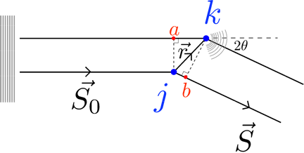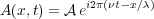
Consider the interaction of a plane wave with two scatterers in a sample, Figure 1. The amplitude of the wave is represented conveniently in the complex notation (we need only the real part) as a function of time and space variables as
where ν is the frequency, λ the wavelength and  is the modulus of absolute value of A(x,t).
Scattering at locations j and k occur without a change of phase, producing an intensity at the detector due to the
combination of the scattered waves. The phase difference between the beams scattered at the two points depends on
the path length difference  -
- . If the vector between the two points is denoted as
  , we see
  is just
  ⋅
⋅ and
and
 is
is  ⋅
⋅ so that the phase difference is
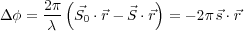
where  = (
= ( -
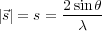
- )∕λ and is referred to as the scattering vector. The magnitude of the scattering vector is related
to the scattering angle as
)∕λ and is referred to as the scattering vector. The magnitude of the scattering vector is related
to the scattering angle as
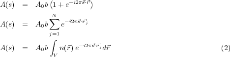
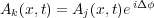
The spherical wave produced by the point scatterer at j is represented by Aj(x,t) = A0bei2π(νt-x∕λ) where A0 is the amplitude of the incident radiation and b is termed the scattering length - it expresses the efficiency or ability of the object to scatter the incident radiation, and has dimensions of length (think about the relationship between the intensity of a spherical wave as dependent on the square of the amplitude, and that of the intensity of a plane wave). The scattered wave at k can be expressed as a phase shift of the scattered wave from j (the two differ only in phase) so
The combination of the scattered waves Aj(x,t) and Ak(x,t) is

The flux is given by the square of the intensity so
We can ignore the x and t dependence and inspect only the scattering vector dependence. It is given in
individual, discrete summation and continuos integral forms in Equation 2 where n( ) is the number of
scatterers within a volume element d
) is the number of
scatterers within a volume element d around
  and
and  is the vector to the jth scatterer from an arbitrary
origin.
is the vector to the jth scatterer from an arbitrary
origin.
From the integral form in Equation 2 we can recognize that the wave amplitude is proportional to the
three-dimensional Fourier transform of the local number density n( ) of scatterers.
A more common notation is much of the x-ray literature is the use of the scattering vector, q given by q = 2πs. The quantity is also defined with respect to wave vectors as

q is also referred to sometimes as the momentum transfer vector since momentum, from the de Broglie equation is p = h∕λ = ℏk and