One vital aspect of manipulation is the analysis of mechanism stiffness. By defining all energetic interactions as energy storage modes, the computation of stiffness is just a matter of computing the Hessian of the robot's summed energy function with respect to the generalized coordinates. This can then be used along with any kinematic constraints on the system to produce a generalized compliance matrix for the mechanism. First, we will zero the forces on the model from the continuing example,
% Zero the force from the previous example.
r.ES_Mode('tip').SetForce([0; 0; 0]);

% Let's assume that the arm is straight out
q2 = zeros(2,1);
The servo stiffness will be defined as a quadratic potential function. A system with infinite steady-state stiffness (such as an integrating controller) can be modeled as a kinematic constraint instead.
% We'll define some servo stiffness for the arm, 100 Nm/rad at each joint
K = 100*eye(2);
r.Add_ES_Mode('servo_stiffness', 'symbolic', 0.5*q.'*K*q);
The compliance of the robot is then found by calling the Compliance method.
% compute the compliance
C = r.Compliance(q2);
We can also compute the compliance at any point from this generalized compliance matrix. Here we will compute the compliance of the manipulator tip with the ComplianceAtPoint method. The first argument is the configuration. The middle argument is a homogeneous transformation object. The last argument is the indices (x and y) to compute
% We can calculate the compliance of the endpoint for this servo stiffness
C_tip = r.ComplianceAtPoint(q2, Link2_Dist, 1:2);
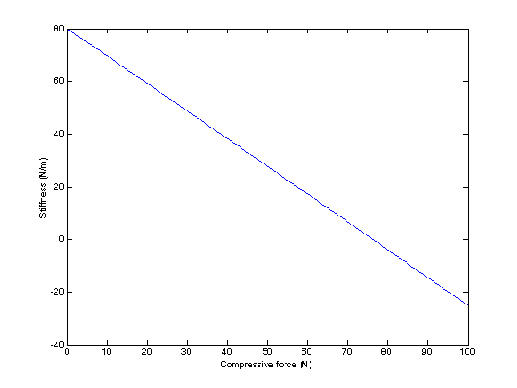
More interestingly, we can examine the effect of arm loading on stiffness. Imagine that the arm is under a constant compression force. This will tend to reduce the stiffness of the arm. By finding the point where the y stiffness of the arm reaches zero, we can find the buckling load of the robot arm in its singular configuration,
% Now let's look for buckling modes.
N = 100;
F = linspace(0, 100, N);
C = zeros(1, N);

for k=1:N
    r.ES_Mode('tip').SetForce([-F(k); 0; 0]);
    C(k) = r.ComplianceAtPoint(zeros(2,1), Link2_Dist, 2);
end

figure(2);
clf;
plot(F, 1./C);
xlabel('Compressive force (N)');
ylabel('Stiffness (N/m)');
The end result looks like the figure below, indicating a buckling force of about 76.4 N.
The script for this tutorial can be downloaded here: tutorial3.txt