In this tutorial, we will demonstrate how to create a two-link planar manipulator, having two 0.5 meter links. To begin constructing a robot in FMAT, place the toolbox files into Matlab's search path. A robot can be instantiated by calling the robot object constructor with a column vector of symbolic variables. In this example, we will use the helpful function make_q, which generates a vector of symbolic variables:
% clear the workspace
clear;

% create a vector of symbolic coordinates for the configuration of the robot
q = make_q(2);

% Instantiate the robot
r = Robot(q);
The kinematics of the robot are constructed using the homogeneous transformation class. To create a coordinate at the origin of the robot, pass the robot in as the first argument to the constructor. The second argument 't' indicates that this is to be a translation, and the third argument specifies a translation of (0, 0, 0) from the origin. The two links are then built up recursively as successive transformations,
% Create an origin for the robot.
Origin = HT(r, 't', [0; 0; 0]);

% Define the link and joint transformations
Link1_Prox = HT(Origin, 'rz', q(1));
Link1_Dist = HT(Link1_Prox, 't', [0.5; 0; 0]);
Link2_Prox = HT(Link1_Dist, 'rz', q(2));
Link2_Dist = HT(Link2_Prox, 't', [0.5; 0; 0]);
Here 'rz' specifies a rotation around the z axis and 't' specifies a translation. This defines the Cartesian kinematics of the manipulator. For the sake of illustration, let's create a crude graphical depiction of this arm. We'll start by placing a 9 cm diameter light blue cylinder at each joint,
% Create some cylinders to represent the joints of the robot arm.
r.Add_DisplayObject('joint1', 'cylinder', [0.2 0.3 1.0], Link1_Prox, 0.1, 0.1, 0.15);
r.Add_DisplayObject('joint2', 'cylinder', [0.2 0.3 1.0], Link2_Prox, 0.1, 0.1, 0.15);
We will also define coordinates of the center of the object, and place rectangles representing each link,
% define the center of each link so we can place a rectangular display
% object there.
Link1_Center = HT(Link1_Prox, 't', [0.25; 0; 0]);
Link2_Center = HT(Link2_Prox, 't', [0.25; 0; 0]);

% Add boxes for the links.
r.Add_DisplayObject('link1', 'box', [0.2 0.3 1.0], Link1_Center, 0.5, 0.08, 0.1);
r.Add_DisplayObject('link2', 'box', [0.2 0.3 1.0], Link2_Center, 0.5, 0.08, 0.1);
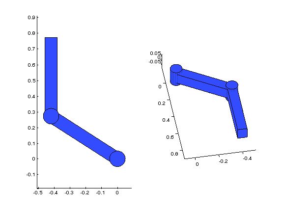
This mechanism can be drawn in any configuration using the Draw method, which takes in as arguments the configuration vector and a figure handle,
% define a configuration, q1
q1 = [pi/2+1, -1];

% create a figure and plot the arm in configuration q1
figure(1);
clf;
subplot(1,2,1)
r.Draw(q1, 1);
axis equal;
subplot(1,2,2)
r.Draw(q1, 1);
axis equal;
view([170 45]);
This should produce a figure similar to this:
This whole example can be downloaded at tutorial1.txt